As of this writing in late-2022, large language models (LLMs) can now easily exceed 10B+ parameters (and the largest at 100B+ parameters). Pure data parallel strategies are no longer viable as the model itself no longer fits on single devices. Fortunately, research and engineering in scaling them have not slowed down; in the JAX (Bradbury et al., 2018) ecosystem in particular we now have pjit, enabling an orthogonal way to parallelize models called tensor parallelism. In this post, we’ll explore the mathematical underpinnings of tensor parallelism, and learn how to implement it for a 15B param language model using pjit.

Intro: Parallelism

Data Parallelism

Until recently, large scale training of deep learning models have primarily used data parallelism:

Each device stores a full copy of the model, and receives a “shard” of the batch (if the full batch is 8 training examples, split along 2 devices each device receives 4 examples).
Each device independently computes the loss, and its gradient (w.r.t. the parameters) using its data shard.
Only once during each step, they synchronize their gradients and update their own copy of the model.

As long as a full copy of the model¹ fits on device, this general strategy can scale gracefully to the typical maximum of 8 GPUs on a single host, and was the likely strategy used to train the “big” (213 million params) Transformer with in the original Attention is All You Need (Vaswani et al., 2017, p. 7) paper ². Properly optimized, data parallelism scales to even hundreds of GPUs on multiple hosts.

However, data parallelism isn’t enough when the model itself can no longer fit on a single device. This is where model parallelism comes in.

Tensor Parallelism

Model parallelism is when we split the model itself across multiple devices. Tensor Parallelism (“sharding”) is one of two ways to do this; the other is Pipeline Parallelism (“pipelining”). The latter is briefly discussed at the end, but the focus here really is on the former.

Tensor parallelism is the answer to this question: what if we could compute the activations of every layer of our model, distributed across all our devices?

Suppose we have 4 devices: with standard data parallelism we make each device compute all the embedding dimensions for 1/4th of the batch:

But perhaps we could make each device compute 1/4th the embedding dimensions for the entire batch, like this:

Even more: instead of sharding on one axis, we could shard both axes. What if we arranged these 4 devices in a \(2\times2\) mesh, such that the first (top left) device computed 1/2 the embedding dimensions for 1/2 the batch?

This is the big idea behind tensor parallelism: arranging our devices into a 2D mesh, and then sharding both our weights and activations on both axes, for all the layers. That is, each device holds a single “shard” of every layer in the model. When done properly, it is possible to run calculations with only one full copy of the model distributed across all the devices.

We’ll start ground up: at the level of the dot products themselves, and see how sharding allows us to do very large matrix multiplies, by trading off increased communication for reduced memory use. Then, we’ll scale it up to a full model in JAX, implementing sharding with pjit on a 15B language model for inference, with focus on the exact code changes, keeping them minimal.

Partitioning: Intuition

Intro: Dot products

Let’s start with an observation: any dot product between two vectors can be broken down into the sum of multiple smaller dot products. Suppose:

\[ a = \begin{bmatrix} 1 \\ 0 \\ 2 \\ -1 \end{bmatrix}, b = \begin{bmatrix} -1 \\ 2 \\ 0 \\ 2 \end{bmatrix} \]

Then, the dot product of these two vectors of length 4 is \[a \cdot b = (1 \times -1) + (0 \times 2) + (2 \times 0) + (-1 \times 2) = -3\]

But we could easily re-write that expanded calculation as \[\textcolor{BurntOrange}{\underbrace{[(1 \times -1) + (0 \times 2)]}_\text{-1}} + \textcolor{Plum}{\underbrace{[(2 \times 0) + (-1 \times 2)]}_\text{-2}}\]

Each of these two terms individually is also a dot product of two vectors of length 2. Recoloring the original vectors, we can imagine them as composed of two “partitioned”-vectors:

\[ a = \begin{bmatrix} \textcolor{BurntOrange}{1} \\ \textcolor{BurntOrange}{0} \\ \textcolor{Plum}{2} \\ \textcolor{Plum}{-1} \end{bmatrix} \;\; b = \begin{bmatrix} \textcolor{BurntOrange}{-1} \\ \textcolor{BurntOrange}{2} \\ \textcolor{Plum}{0} \\ \textcolor{Plum}{2} \end{bmatrix} \]

Now, say I wanted my friend to help out with this tedious calculation. If I calculated the dot product with the first partition of each vector (getting back \(\textcolor{BurntOrange}{-1}\)), they’d only need to return the result (\(\textcolor{Plum}{-2}\)) of their partition (and not their entire sub-vectors) for me to calculate the full dot product, \((-1)+(-2)=-3\).

Intro: Matrix multiplies

Let’s build on this with another observation: In a matrix multiply \(AB=C\), \(C\) is simply a storage mechanism for the pairwise dot-products of all the (row) vectors of \(A\) and (column) vectors of \(B\)³. Specifically, let:

\[A = \begin{bmatrix} \textcolor{LimeGreen}{1} & \textcolor{LimeGreen}{0} & \textcolor{LimeGreen}{2} & \textcolor{LimeGreen}{-1} \\ 2 & 1 & 0 & -2 \end{bmatrix} \;\; B = \begin{bmatrix} 0 & \textcolor{LimeGreen}{-1} \\ 1 & \textcolor{LimeGreen}{2} \\ 2 & \textcolor{LimeGreen}{0} \\ 0 & \textcolor{LimeGreen}{2} \end{bmatrix}\;\; AB = C = \begin{bmatrix} 4 & \textcolor{LimeGreen}{-3} \\ 1 & -4 \end{bmatrix} \]

\(A\)’s first row vector and \(B\)’s second column vector should seem familiar: we just took their dot products. And as expected, the element of the first row, second column of \(C\) is that dot product \(-3\). This perspective also neatly explains two facts about matrix multiplication:

Why \(C\) is a \(2 \times 2\) matrix: \(A\) has two row vectors, and \(B\) has two column vectors, resulting in a \(2 \times 2\) matrix to capture all the pairwise dot products. (Likewise, if \(A\) had \(3\) row vectors, \(C\) would be of shape \(3 \times 2\)).
Why the “inner axes” (\(A\) being \(2 \times \textcolor{LimeGreen}{4}\), \(B\) being \(\textcolor{LimeGreen}{4} \times 2\)) have to match: we can’t take dot products of vectors of different lengths. Take note of this “inner axes” terminology, we’re about to build on this right now!

Both combined, we have the general rule for the shapes: \(\underbrace{A}_{n\times d} \underbrace{B}_{d\times m} = \underbrace{C}_{n\times m}\)

Sharding: A Matrix Multiply

The vast majority of compute time in deep neural networks is spent on the matrix multiplies (matmuls) between data (activation) matrices and weight matrices. We focus on a single matmul in this section, building up two cases (1A, 1B and 2), that together can explain every possible sharding pattern.

Let’s start:

Suppose we now have a new \(A\) matrix of shape \(4 \times 16\), and a \(B\) matrix of shape \(16 \times 4\). That is, each has 4 vectors of length 16 each. We want to compute \(C=AB\), where \(C\) will be a \(4\times4\) matrix.

Also suppose we have 8 GPUs/TPUs, which are much slower at multiplying matrices than adding matrices⁴. We arrange these 8 devices in a \(2\times4\) mesh.

Our goal here is to do as little compute as possible here: in the final version, we should split up this large matrix multiply such that we only compute one full copy of \(C=AB\) split across all 8 devices.

Case 1: Inner Axes

For now, let’s try a version of the problem that may be easier to reason about: split up \(AB\) such that each device has one full copy of \(C=AB\).

To get started, we can partition both matrices, just as we previously partitioned vectors. Note that unlike vectors, with matrices we have multiple axes we can “slice” on. For now, let’s use this pattern, where each “sub-matrix” is a \(4\times 4\) matrix:

Since \(A\) is the first matrix (row vectors) and \(B\) is the second matrix (column vectors) in the matmul \(AB\), we’re effectively partitioning along the “inner axes”; cutting each vector into multiple sub-vectors, just as in the dot product example. To make this clearer, we might write down this “sharding configuration” in pseudocode as:

\(A\): (full, sharded)
\(B\): (sharded, full)

Continuing this reasoning, just as we decomposed the large dot product into the sum of multiple smaller dot products, we can decompose this larger matrix multiply into the sum of smaller matrix multiplies. Specifically, \(AB = A_1B_1+A_2B_2+A_3B_3 +A_4B_4= C_1 + C_2 + C_3+C_4\).

Each of these terms is the pairwise dot product of a subset of \(A\) and \(B\)’s vectors’ feature dimensions; \(C_1 = A_1B_1\) is the matrix holding the pairwise dot products of the vectors’ first four dimensions, \(C_2 = A_2B_2\) is the second four, and so on. Summing the four \(C_i\) matrices, we have the pairwise dot products computed along all the vector dimensions.

This result implies something curious: to multiply a \(4 \times 16\) and \(16 \times 4\) matrix, we don’t need to do it in one go; we can just do \(4 \times 4\) multiplies and add the results. If we did these multiplies on different devices, that’s a neat way of speeding up the multiplication, and that’s the idea at the heart of tensor parallelism. There’s two possible cases here: when the sharding axes “match”, and when they “mismatch”, both of which will appear in the full neural network we’ll examine.

Case 1A: Mesh-axes match

Since we have a \(2\times4\) device mesh, one way to partition \(A\) and \(B\) onto this mesh is the following way:

In technical terms, \(A\)’s column dimensions and \(B\)’s row dimensions are sharded along the Y axis. We could write our sharding config now as:

\(A\): (full, sharded_Y)
\(B\): (sharded_Y, full)

This config concisely captures how the matrices are divided across this mesh. For instance, on the four devices where X=0 (the top row), we have all of \(A\)’s rows (first axis), and the second shard of \(A\)’s columns (the second axis; here, the second 4 dimensions). A full copy of \(A\) then is distributed across Y=0,1,2,3.

However, there’s duplication: since we’re not sharding on X, it means there are two full groupings with Y=0,1,2,3, each with a full copy of \(A\). The same reasoning applies to \(B\) (as we see in the diagram), but with rows and columns reversed.

Multiply

Now, each device multiplies the shard of \(A\) and \(B\), to produce part of the multiplied value \(C\). For example, the device at X=0, Y=1 on the mesh produces \(C_2 = A_2B_2\).

Note that the duplication over the X axis results in both duplicate memory use and computation: for instance, both X=0, Y=0 and X=1, Y=0 are performing the same calculation.

AllReduce

All these matmuls are only fragments of \(C\): they have the same shape as \(C\), but each only contains pairwise dot products of parts of \(A\) and \(B\)’s vectors. To calculate the full \(C\), the devices can “pull” the other necessary values from its neighbors and then add them to its own calculation. These collective ops are well known, and this specific one is called AllReduce⁵. Let’s visualize this from X=0, Y=1’s perspective (but remember, for now and the rest of this post, in actuality collective ops are performed by all devices at the same time):

To recap, our starting scenario was one where each device had to perform this \((4\times 16) \times (16 \times 4)\) matrix multiply to get a copy of the final result \(C\). With sharding, each device only had to do one \((4\times 4) \times (4\times 4)\) matrix multiply, and sum together the partial results from its neighbors.

And here’s the real lesson: this “shard \(\rightarrow\) multiply \(\rightarrow\) allreduce” strategy scales to far larger matrices! If in the self-attention block of a Transformer we had \(Q\) and \(K\) matrices of shape \(512 \times 4096\) each (\(512\) vectors, each of length \(4096\)), then getting the “match” between every pair of queries and keys \(QK^T\) is a \((512 \times 4096) \times\) \((4096 \times 512)\) matrix multiply.

With this strategy, by splitting the inner axes along the mesh Y axis’s 4 devices, each device in the group of 4 only has to do a \((512 \times 1024) \times\) \((1024 \times 512)\) multiply (that is, pairwise dot products with just 1024 of 4096 dimensions each), which is about 4x faster⁶.

But we’re still duplicating work along the X axis; we’ll see shortly how with Case 2, this can be this 8x faster, leveraging all 8 devices.

Case 1B: Mesh-axes mismatch

Let’s try the above problem (each device obtains a full copy of \(C\)), with a modified sharding config:

\(A\): (full, sharded_Y)
\(B\): (sharded_X, full)

That is, we now shard \(B\)’s first axis on X, not Y. Visualized, the mesh now looks like this:

This doesn’t appear to be a very useful mesh: we now have 4 copies of \(B\) over the mesh, compared to the previous two. Worse, because the sharding axes mismatch, we can’t actually multiply: \(A_1\) is of shape \(4\times4\) (since 16 divided on 4 devices), and \(B_1\) is of shape \(8 \times 4\) (16 divided on 2 devices). That is, their number of inner dimensions don’t match: each device has twice as many dimensions of \(B\)’s (column) vectors than they have of \(A\)’s (row) vectors.

This inability to multiply will be true in general: assume we start off with a valid matmul (inner axes match in number of dimensions), we’re dividing this inner axis length by the number of devices on the corresponding mesh axis, and that may not be the same. Here, \(A\) does \(\frac{16}{4}=4\) due to the four devices on Y, while \(B\) does \(\frac{16}{2}=8\) due to the two devices on X.

But this is fine: we can use another collective op called AllGather, to restore the full matrices on each device. Visualizing this on X=0, Y=1 (and remembering that in reality all devices are doing this at the same time):

Once each device restores a full copy of \(A\) and \(B\), they multiply it as normal to directly get \(C\). Now, this may seem odd: why’d we shard the matrix, only to gather it (then multiply) in full on every single device? (that is, no compute benefit, since every device does the same calculation).

Because it turns out when we combine Case 1B with Case 2, we can quite cleanly eliminate this duplicate computation. Let’s see how.

Case 2: Outer Axes

We’ve focused on sharding on the “inner axes” of a matrix multiply so far, but there’s nothing stopping us from sharding the outer axes; if anything, it’s easier! Building on prior examples, let’s try this sharding pattern:

\(A\): (sharded_X, sharded_Y)
\(B\): (sharded_X, full)

Visualizing, we have the following:

Since there’s a *lot* of partitions this point on, it’s easier to keep track of them by keeping track of their “colored in” areas than naming them individually.

This is still the same as case 1B, with one change: A’s outer axis is now sharded on X. This means that devices with X=0 contain shards of the first 2 (of 4) row vectors, whereas devices where X=1 contain shards of the second 2 (of 4) vectors. The feature dimensions of these vectors remain sharded over Y.⁷ We now only have one full copy of \(A\), fully distributed over the entire \(2\times4\) mesh.

We now proceed as previously with case 1B, allgathering \(A\) and \(B\) on their inner axes. Visualizing from the perspective of X=0,Y=1:

Now we multiply the first 2 (of 4) row vectors of \(A\) with the 4 column vectors of \(B\). To store these pairwise dot products, we end up creating a \(2\times4\) matrix, that is, the top half of the (final) values of \(C\):

Once all 8 devices do their respective allgathers and multiplies, we have:

This should feel familiar! If \(A\) is a batch of data (what we’d typically call \(X\)), with individual training examples as row vectors, then this is just batch parallelism: the two “submeshes” (corresponding to X=0 and X=1) are each processing half of this batch, and then store the half of \(C\) that corresponds to the shard of \(A\) it processed.

But there’s still duplicate computation going on: all four devices in the submesh (X=0 or X=1) are doing the same work!

Full Sharding

What if we also sharded \(B\) along its outer axis? That is, we shard both \(X\) and \(Y\) over X and Y, with the following sharding pattern:

\(A\): (sharded_X, sharded_Y)
\(B\): (sharded_X, sharded_Y)

Visualized, we see that we only have one copy of \(A\) and \(B\) distributed over the whole mesh:

Since this sharding spec produces a mismatch along the inner axes, using case 1B, we do an all gather. However, this time as we’ve also sharded both the outer axes, X=0,Y=1 will only be processing the full pairwise dot products of the first shard (first 2 row vectors) of \(A\), with the second shard (the 2nd column vector) of \(B\).

And then, a multiply, resulting in a \(2 \times 1\) shard of the final output:

Zooming out, we see all 8 devices have computed a unique part of the output. Even more wonderfully, \(C\) has the same sharding pattern as \(A\) and \(B\), (sharded_X, sharded_Y):

Sharding: GSPMD-style

The GSPMD paper (Xu et al., 2021) introduced an optimal sharding pattern for Transformers, subsequently used to train PaLM (Chowdhery et al., 2022). To reinforce our understanding of the two cases above, we’ll now look at the sharding spec for the feedforward network in the Transformer layer. But before that, one final detour:

GSPMD is the parallelization system that enables pjit, implemented as an extension to XLA (JAX’s compiler).

What is \(XW\)?

Deep learning models at their core are straightforward: a number of layers stacked on top of each other. The core building block is the fully connected layer, often written as \(\sigma(XW + b)\). It’s really three operations:

\(XW\)⁸ is a matrix multiply, where \(X\) is a matrix of datapoints as row vectors, and \(W\) is a weight matrix.
\(b\) is a vector of biases we add to \(XW\).
\(\sigma\) is a non-linearity of our choice, often ReLU but more recently enhanced variants such as GeLU in Transformer models.

We know what it means to shard the data \(X\) along its outer axis over X: it’s just splitting the batch into yet smaller batches, standard data parallelism. But what does it mean to shard \(W\) along its outer axis, over Y? To understand that, let’s dive deeper: what is \(XW\)?

Well, it’s just a storage mechanism for the dot products of \(X\)’s row vectors, and \(W\)’s column vectors. We can directly reuse the math at the start of this post, replacing \(A\) and \(B\) with \(X\) and \(W\):

\[X = \begin{bmatrix} \textcolor{LimeGreen}{1} & \textcolor{LimeGreen}{0} & \textcolor{LimeGreen}{2} & \textcolor{LimeGreen}{-1} \\ 2 & 1 & 0 & -2 \end{bmatrix} \;\; W = \begin{bmatrix} 0 & \textcolor{LimeGreen}{-1} \\ 1 & \textcolor{LimeGreen}{2} \\ 2 & \textcolor{LimeGreen}{0} \\ 0 & \textcolor{LimeGreen}{2} \end{bmatrix}\;\; XW = \begin{bmatrix} 4 & \textcolor{LimeGreen}{-3} \\ 1 & -4 \end{bmatrix} \]

The first row of the output matrix, stores the dot products of the first row vector of \(X\) with all of the column vectors of \(W\). Since the dot product calculates how much two vectors “match” ⁹, the new output row vector (of the \(XW\)) stores how much the original row vector (of \(X\)) matches with each of the \(W\) weight vectors. Since we have two weight vectors, the output row vectors have two feature dimensions; if we have 20,000 weight vectors, they’d have 20,000 feature dimensions!

This output, once passed through a nonlinearity are the new data vectors (the “activations”), which will then be multiplied with the next layer’s weight matrix to produce yet newer activations. This really is what we mean by stacking layers on top of each other: using the feature matching scores of one layer as the data to the next layer.

Answering the question, to shard \(W\)’s outer axis along Y is to ask each device with a given Y value to compute the dot products with a subset of \(W\)’s column vectors. We can do this since the dot product of a data vector with a weight vector doesn’t depend on any other weight vectors. This means on a \(2\times4\) mesh with Y=0,1,2,3, devices with Y=0 can calculate dot products with the first 1/4th of the weight vectors, devices with Y=1 the second 1/4th, and so on. This is exactly what we see in the calculation of \(C\) in the previous section (again, replace \(A\) and \(B\) with \(X\) and \(W\))

GSPMD’s sharding spec

To recap, in the original Transformer (and most variants since), “Each layer has two sub-layers. The first is a multi-head self-attention mechanism, and the second is a simple, position-wise fully connected feed-forward network.” (A. Huang et al., 2022) Let’s look at the GSPMD paper’s proposed sharding spec for the second sub-layer, the feedforward network (FFN):¹⁰

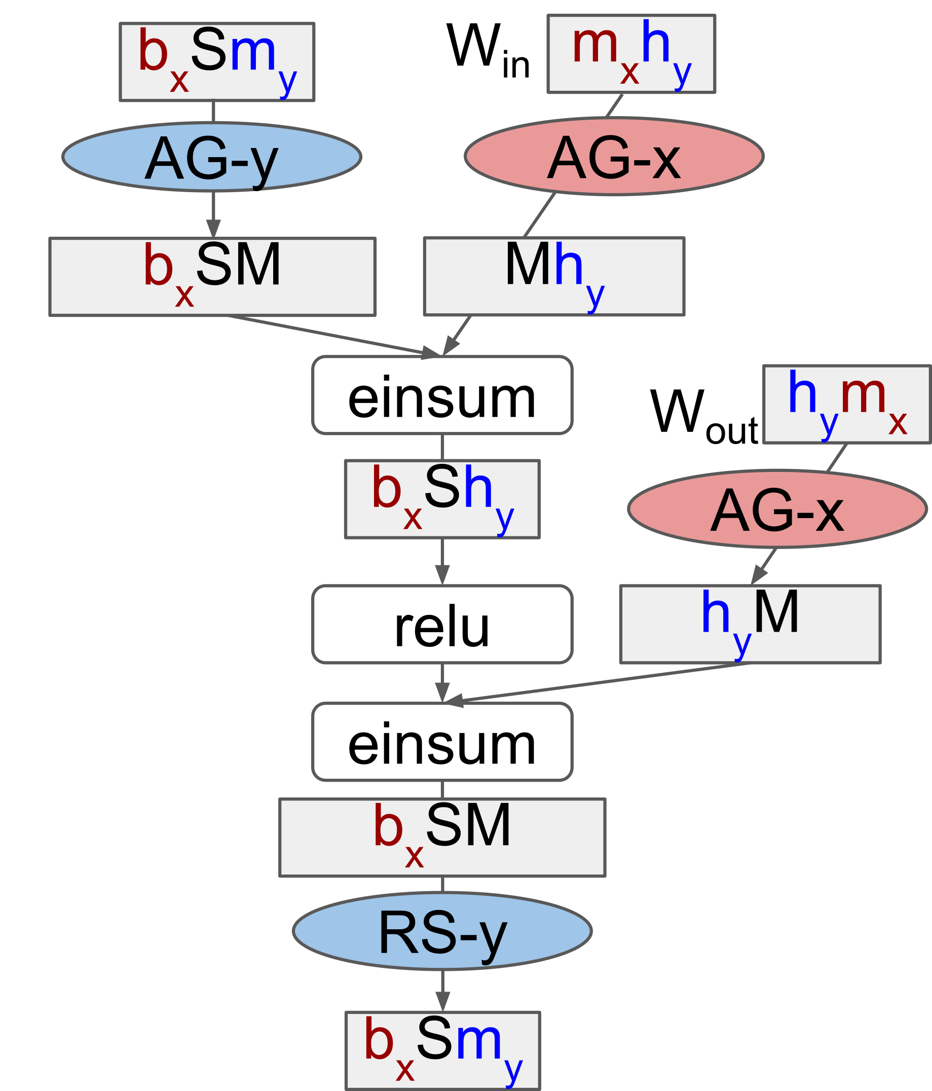
Fig. 7 from the GSPMD paper, modified with data \(X\) on the left (weight \(W_{\text{in}}\) on the right) to emphasize the \(XW_{\text{in}}\) matmul

The FFN is made of two fully-connected layers (the \(\sigma(XW + b)\) we just discussed). Breaking this down:

The first multiplies a weight (\(W_{\text{in}}\), sharded as \(\textcolor{Maroon}{m_x}\textcolor{Blue}{h_y}\)) to transform the input features (the original embeddings, sharded as \(\textcolor{Maroon}{b_x}S\textcolor{Blue}{m_y}\)) into the features of the “hidden layer” (sharded as \(\textcolor{Maroon}{b_x}S\textcolor{Blue}{h_y}\)). In most implementations, the hidden layer has 4x the number of features of the input/outputs of the FFN.
The second multiplies a weight (\(W_{\text{out}}\), sharded as \(\textcolor{Blue}{h_y}\textcolor{Maroon}{m_x}\)) to transform the features of the “hidden layer” (sharded as \(\textcolor{Maroon}{b_x}S\textcolor{Blue}{h_y}\)) into the output features (the new embeddings, sharded as \(\textcolor{Maroon}{b_x}S\textcolor{Blue}{m_y}\)). The number of output features are the same as the input features, but the features themselves are different!

Let’s zoom in on this, looking at each of these multiplies (the einsums in the diagram) separately:

Embed \(\rightarrow\) Hidden

To make things concrete, let’s say we have \(8\) sequences, each of length \(512\), and an embedding dimension of \(5120\). That is, the shape of \(X\) is \((B \times S \times M)\)\(=(8 \times 512 \times 5120)\). Since we want 4x the number of features for the hidden layer, we’ll need \(20480\) weight vectors of length equalling the embedding dimension \(5120\); hence \(W_{\text{in}}\) is of shape \((M \times H)\)\(= (5120 \times 20480)\).

The sharding spec for the data \(X\) and weights \(W\), in the concise form in the diagram are \(\textcolor{Maroon}{b_x}S\textcolor{Blue}{m_y}\), and \(\textcolor{Maroon}{m_x}\textcolor{Blue}{h_y}\). We can rewrite this more verbosely as:

\(X\): (shard_X, full, shard_Y) # (batch, seq_len, embed)
\(W\): (shard_X, shard_Y) # (embed, hidden)

Note that we don’t shard along the sequence length axis. This means, for instance, device X=0, Y=1 has:

the second of four slices (the second \(1280\) of \(5120\)) along the embedding dimension
of all the timesteps
of the first of two slices (the first \(4\) of \(8\)) along the batch dimension.

This sharding pattern should look familiar: this is Case 2 (since the outer axes are sharded) combined with Case 1B (since the inner axes are sharded on mismatched mesh axes), again! Visualizing again from the perspective of X=0, Y=1:

As previously in Case 1B, we allgather the first matrix (here, \(X\)) along Y, and the second matrix (here, \(W_{\text{in}}\)) along X. Once allgathered, both matrices have their inner axes = \(M = 5120\) dimensions.

We leave the outer axes sharded: this means we’re only multiplying the embeddings of the first 4 (of 8) sequences in the batch. We’re multiplying all the input dimensions, but only computing the second (of four slices) of the hidden dimensions, that is, dimensions (5120, 10239) of \(20480\) dimensions.

All 8 devices then compute a unique shard of the output (corresponding to a different batch slice along X, and hidden dimension slice along Y), successfully avoiding any duplications.

Hidden \(\rightarrow\) Embed

So far, it seems like we’ve only been using Case 1B and Case 2. But here, the sharding spec for the data and weight, in the concise form are \(\textcolor{Maroon}{b_x}S\textcolor{Blue}{h_y}\) and \(\textcolor{Blue}{h_y}\textcolor{Maroon}{m_x}\). In verbose form:

\(X\): (shard_X, full, shard_Y) # (batch, seq_len, hidden)
\(W\): (shard_Y, shard_X) # (hidden, embed)

That is, the inner axes are sharded on the same mesh axis, which is case 1A. This means we can directly multiply on-device (without having to allgather over the inner axes), and then run allreduce to get the final output. There is one problem though: when both matrices are fully sharded over a 2D mesh, and the mesh axes of their inner axes match, the mesh axes of their outer axes also match.

This means if we multiply the shards directly, we’ll have the opposite problem of duplicate work: incomplete work. Specifically, since both the outer axis of \(X\) (batch) and \(W_{\text{out}}\) (embed) are sharded on X, for the first batch slice on the X=0 submesh we’ll only compute the dot product with the first half of the weight vectors (on X=1, the dot products of the second batch slice with the second half of the weight vectors).

We don’t have any devices computing the dot products of the first batch slice with the second half of weight vectors (and vice versa)!

To fix this, we need to allgather either \(X\) or \(W\) across their outer axis. Generally, we prefer to keep the batch axis sharded, so we allgather along \(W\)’s outer axis. This means each device now computes:

the dot product over 1/4th of the hidden dimensions
for 1/2 of the batch
for all of the weight vectors.

Then multiplying, each device along X=0 produces part of the dot products for all the embedding dimensions (case 1A), for the first batch shard (case 2):

At this point, we have two options: we can either proceed with an allreduce, as previously covered in case 1A. Or, we can notice what we want is to produce an output tensor with the same sharding pattern as the input to the entire FFN subnetwork. In this case, we can use a different collective op called reduce-scatter. Unlike allreduce, which sums up values across all devices for the entire shard, this sums up values only for the smaller part of the shard we want:

Wrapping it up

We did it! As we see, Case 2, combined with Case 1A or 1B as appropriate allowed us to stack two fully sharded, fully connected layers on top of each other, and produce an output with the exact same sharding as the input (no resharding needed!).

We won’t cover the sharding of the self-attention sublayer here, but you should be able to combine the two cases here, with Table 1 in the GSPMD paper to work out how the attention heads are sharded over the Y axis¹¹.

Partitioning: In JAX

Now that we have a deep understanding of how to shard a neural network, let’s write some code! We’re in luck here: I’m currently working on a port of the ESM2 (Lin et al., 2022) protein language model into Flax (Heek et al., 2020), so much of the examples will be directly pulled from the working codebase.

For context: the model built here is a BERT (Devlin et al., 2019) style, encoder-only Transformer. It is a 15B param model with 48 layers, and 5120 dimensional embeddings as seen in the previous section. Each encoder layer has two sublayers as previously described: a self-attention sublayer followed by a feedforward network sublayer. Let’s start by understanding pjit’s programming model, then using it to progressively build the full model.

The `pjit` programming model

A good way to think of pjit is a supercharged jax.pmap. If you recall, pmap runs the same program on multiple devices, each with a different shard of input data over the batch axis. pjit is more flexible: it allows us to shard both the data and weights (and when training, even the optimizer states) in whatever configuration we please over a mesh. To do so, pjit requires three things from us:

A mesh specification, mapping the “logical” devices on the 2D (or higher-D) mesh to the physical devices available.
The sharding spec of all tensors being passed as input to, and returned as output to from the function.
Sharding constraints for select intermediate tensors inside the function. This isn’t strictly necessary (XLA GSPMD will try to find a viable layout), but can lead to improved memory usage.

Note what isn’t here: JAX doesn’t need us to insert any of the collective ops we discussed. It uses a constraint based model, where we specify sharding constraints for the “big”, memory intensive tensors, and it automatically determines the sharding pattern for all other intermediate tensors in the function, as well as any collective ops that need to be inserted to meet these constraints.

Sharding constraints

So how do we specify a sharding constraint? Well, we write our function as we normally would, and then call with_sharding_constraint on the tensor we’d like to place the constraint on:

Note this is flax’s version of the method, which comes with nice add-ons such as checking if we’re inside a pjit and rule translation. jax has a more direct version here.

from flax.linen import partitioning as nn_partitioning

def forward(x):
    # ...run some code here.
    # note x here has shape [batch x seq_len x embed]
    x = nn_partitioning.with_sharding_constraint(x, ("batch", None, "embed"))
    # ...continue more code here.
    return x

When not inside a pjit, this is a no-op, returning the original input unchanged. Inside a pjit, XLA will insert any collective ops needed to meet the constraints we specified in the second argument.

The second argument here specifies the mesh axis to shard each of the axes of this rank-3 tensor over. The None in the middle means “do not shard over the sequence length axis”. But note that the other two don’t have X or Y, but “names” (batch and embed). This is because at runtime, we’ll use a set of rules mapping these from names to the mesh axes. For instance, here’s the one I use for the ESM2 models on a \(2 \times 4\) mesh:

# Create 2D TPU mesh
DEFAULT_TPU_RULES = [
    ("batch", "X"),
    ("hidden", "Y"),
    ("heads", "Y"),
    ("embed_kernel", "X"),
    ("embed", "Y"),
]

Under these rules, ("batch", None, "embed") will become ("X", None, "Y"). Writing our code this way keeps it flexible as we potentially try out different sharding configurations.

A first run

Then, at runtime there’s three things we need to do:

Create the mesh: the mesh is the object that translates our abstract, 2D mesh to the actual physical hardware that will be running the computation. This is where we specify, say, which of the 8 physical devices becomes the mesh device X=0,Y=1.

from jax.experimental import maps

mesh_shape = (2, 4)
# We reshape the devices into a 2D mesh, and name the mesh axes.
devices = np.asarray(jax.devices()).reshape(*mesh_shape)
mesh = maps.Mesh(devices, ("X", "Y"))

pjit the function: This is similar to jax.jit, except we now also need to specify the sharding spec for the input and output.

The input to this transformer is, say, a \(8 \times 512\) matrix of integers, and we shard the first (batch) axis along the mesh X axis.
The output is \(5120\) dimensional vectors, so the output is a matrix of shape \(8 \times 512 \times 5120\). We keep the batch axis sharded over X, and the embedding axis sharded over Y, which we define as P("X", None, "Y"). Note that pjit is lower level than the flax methods, and needs the mesh axes directly inside a PartitionSpec; the translation rules we define above are only used for the constraints inside the nn.Module. You can read more about pjit at the JAX level here.

from jax.experimental import pjit, PartitionSpec as P

# Create fn for inference.
pjit_forward = pjit.pjit(
    forward,
    in_axis_resources=P("X", None),
    out_axis_resources=P("X", None, "Y"),
)

Call the function: we use two context managers, one to activate the mesh, and the other specifying the translation rules for all the sharding constraints inside the function.

with maps.Mesh(mesh.devices, mesh.axis_names), nn_partitioning.axis_rules(
    DEFAULT_TPU_RULES
):
    x = pjit_forward(x)

Let’s now apply these constraints to the weights and activations of the feedforward network.

Applying constraints to a FFN

In a previous section, we looked at the sharding spec the GSPMD paper proposed for the FFN in a transformer layer. To summarize in a table:

The full sharding spec for both the FFN and self-attention can be found in Table 1 in the GSPMD paper. PaLM uses this same spec, but over a much larger \(256\times12\) mesh per pod. (Sec. 4)

Tensor	Sharding Spec `[shape]`
\(\text{activation: embedding}\)	\(X, \_, Y\) `[batch, seq_len, embed]`
\(W_{\text{in}}\)	\(X, Y\) `[embed, hidden]`
\(\text{activation: hidden}\)	\(X, \_, Y\)`[batch, seq_len, hidden]`
\(W_{\text{out}}\)	\(Y, X\) `[hidden, embed]`

This sharding spec is for any generic, dense Transformer. The code below is the second sublayer (the FFN network) of an encoder layer in the ESM2 model. We apply this sharding spec to the weights on lines 11 and 21, and to the activations on lines 13 and 23:

# ... we apply a layer norm and multi-head attention before this.

# Create second residual block (LayerNorm + MLP)
residual = x
x = nn.LayerNorm(name="final_layer_norm", epsilon=1e-5)(x)

# Create + apply first MLP layer with weight + activation sharding constraints.
x = partitioning.Dense(
    self.ffn_embed_dim,
    name="fc1",
    shard_axes={"kernel": ("embed_kernel", "hidden")},
)(x)
x = nn_partitioning.with_sharding_constraint(x, ("batch", None, "hidden"))
# Don't approximate gelu to avoid divergence with original PyTorch.
x = nn.gelu(x, approximate=False)

# Create + apply second MLP layer with weight + activation sharding constraints.
x = partitioning.Dense(
    self.embed_dim,
    name="fc2",
    shard_axes={"kernel": ("hidden", "embed_kernel")},
)(x)
x = nn_partitioning.with_sharding_constraint(x, ("batch", None, "embed"))
x = residual + x

return x

The activation sharding specs are applied as in the initial example: we just with_sharding_constraint. But there’s two new things:

There’s a new shard_axes argument being passed into the layer definition on lines 11 and 21.
We’re using the partitioning.Dense layer instead of the standard nn.Dense.

Let me elaborate on what’s going on here.

Sharding constraints: Weights

Here’s the goal: we want to apply the same with_sharding_constraint function we used on the activation tensors, to the weight tensors in these Dense layers. Problem is, it’s defined as a local variable inside the __call__ method of nn.Dense; and is not an attribute I can access from the outside. There’s two options here:

First is the t5x (Roberts et al., 2022) route of creating a new version of Dense directly with the constraint applied inside the __call__ method. This works in a robust, well-tested library! However, we’d need to make a modified copy of every layer where we want to apply a constraint over a weight.
The second approach is noticing that all flax.linen layers use the nn.Module’s (their parent class) .param method to create their params. Then, we can write a simple mix-in class that overrides the default param method to apply the sharding right as it is created:

@dataclasses.dataclass
class ShardMixIn:
    """Adds parameter sharding constraints for any flax.linen Module.
    This is a mix-in class that overrides the `param` method of the
    original Module, to selectively add sharding constraints as specified
    in `shard_axes`"""

    shard_axes: Optional[Mapping[str, Tuple[str, ...]]] = None

    # Modifies off 
    # https://github.com/google/flax/blob/main/flax/linen/partitioning.py#L304
    def param(self, name: str, *init_args):
        # Initialize using the original Module's `param` method
        param = super().param(name, *init_args)

        # If `shard_axes` specified and param name in the dict, apply constraint
        if self.shard_axes and (name in self.shard_axes.keys()):
            axes = self.shard_axes[name]

            # Apply the sharding constraint (e.g. axes=('embedding', 'hidden'))
            param = nn_partitioning.with_sharding_constraint(param, axes)

            # Sow this, to have the AxisMetadata available at initialization.
            self.sow(
                "params_axes",
                f"{name}_axes",
                nn_partitioning.AxisMetadata(axes),
                reduce_fn=nn_partitioning._param_with_axes_sow_reduce_fn,
            )

        return param

There’s only 10 lines of code here, which add the shard_axes argument to any Flax nn.Module. As we can see, with_sharding_constraint is applied on line 21, only when a given param has a constraint specified. No need to rewrite the original layer definition, we simply create a new version that inherits the original, and our mix-in:

class Dense(ShardMixIn, nn.Dense):
    pass

This is just one solution to be able to apply with_sharding_constraint to the weights, and I’m definitely quite open to feedback on whether this is a sensible strategy!

Putting it all together

We omitted a key detail in the opening example: in the real forward pass (the .apply method) we need to pass in both esm_sharded_params, and the data batch. Since the params are an input argument, they will also need a sharding spec. The params in Flax are a PyTree (specifically, a nested dict) and so the sharding spec is a nested dict with the same structure. There’s some plumbing here, so let’s go through it step by step:

Because the ShardMixIn .sow’s the sharding metadata into the module, this metadata is available at model initialization with the .init method. Let’s initialize the 15B model, and inspect the shapes of the parameters of layer 42:

Code

import functools
import flax.linen as nn
import jax
import jax.numpy as jnp

from esmjax.modules import modules
from esmjax.modules import partitioning


embed_dim = 5120
num_heads = 40
num_layers = 48

embedding = nn.Embed(33, embed_dim)
block_fn = functools.partial(modules.EncoderLayer, num_heads, embed_dim, embed_dim * 4)
esm2 = modules.ESM2(embedding, block_fn, num_layers)

key = jax.random.PRNGKey(0)
arr = jnp.array([[0, 1, 2]])

We can see that the 5120-dimensional embeddings are projected to produce embeddings for 40 heads, with 128 dims each.

# jax.eval_shape replaces all actual arrays with ShapeDtypeStruct
# This avoids memory use, *and* allows us to inspect the param shapes.
params = jax.eval_shape(esm2.init, key, arr)
params['params']['42']['self_attn']

FrozenDict({
    k_proj: {
        bias: ShapeDtypeStruct(shape=(40, 128), dtype=float32),
        kernel: ShapeDtypeStruct(shape=(5120, 40, 128), dtype=float32),
    },
    out_proj: {
        bias: ShapeDtypeStruct(shape=(5120,), dtype=float32),
        kernel: ShapeDtypeStruct(shape=(40, 128, 5120), dtype=float32),
    },
    q_proj: {
        bias: ShapeDtypeStruct(shape=(40, 128), dtype=float32),
        kernel: ShapeDtypeStruct(shape=(5120, 40, 128), dtype=float32),
    },
    v_proj: {
        bias: ShapeDtypeStruct(shape=(40, 128), dtype=float32),
        kernel: ShapeDtypeStruct(shape=(5120, 40, 128), dtype=float32),
    },
})

We can also see the axis metadata generated when calling the .init method:

params['params_axes']['42']['self_attn']

FrozenDict({
    k_proj: {
        kernel_axes: AxisMetadata(names=('embed_kernel', 'heads', None)),
    },
    out_proj: {
        kernel_axes: AxisMetadata(names=('heads', None, 'embed_kernel')),
    },
    q_proj: {
        kernel_axes: AxisMetadata(names=('embed_kernel', 'heads', None)),
    },
    v_proj: {
        kernel_axes: AxisMetadata(names=('embed_kernel', 'heads', None)),
    },
})

Only the params that we’ve specified a sharding constraint over exist in this PyTree. To pass into pjit, we use a utility function to convert the names into mesh axes, and replicate the structure of the full params. The AxisMetadata are replaced with proper PartitionSpecs, and all other params have their sharding pattern set to None, meaning full replication.¹²

params, params_axes = params.pop("params_axes")
esm_axes = partitioning.get_params_axes(params, 
        params_axes, 
        rules=partitioning.DEFAULT_TPU_RULES)
esm_axes['params']['42']['self_attn']

FrozenDict({
    k_proj: {
        bias: None,
        kernel: PartitionSpec('X', 'Y', None),
    },
    out_proj: {
        bias: None,
        kernel: PartitionSpec('Y', None, 'X'),
    },
    q_proj: {
        bias: None,
        kernel: PartitionSpec('X', 'Y', None),
    },
    v_proj: {
        bias: None,
        kernel: PartitionSpec('X', 'Y', None),
    },
})

We now pass this sharding spec (esm_axes) into the pjit definition. Then, we have a fully sharded inference method, distributing the computation work of this 15B model across all 8 cores of a TPU. You can find a fully runnable notebook here.

apply_fn = pjit.pjit(
    esm.apply,
    in_axis_resources=(esm_axes, P("X", None)),
    out_axis_resources=P("X", None, "Y"),
)

with maps.Mesh(mesh.devices, mesh.axis_names), nn_partitioning.axis_rules(
    partitioning.DEFAULT_TPU_RULES
):
    embeds = apply_fn(esm_sharded_params, batch)

Program Trace

Upto now, we’ve handwaved the fact that there’s a lot of communication going on in this forward pass. How much time on the forward pass are we spending on these collective communication ops? The short answer: on a TPUv2-8, about 20%¹³. The way to answer this is a program trace, and JAX makes this easy: here’s the full trace of all 48 layers of the ESM2 15B model on TPU3 (of 0 to 7) of a TPUv2-8, taking about 4.25s to complete inference with a batch size of 32:

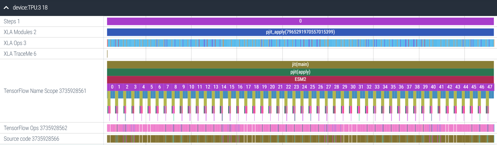
Let’s zoom in on layer 42. We can tell from this trace that the FFN sublayer (fc1 and fc2) takes more time to execute than the self-attention sublayer. On the top bar we have the XLA Ops, the direct, device-level ops being executed. Most of these are fusion ops, a combination of fused multiplies and elementwise ops (e.g. addition, subtraction):

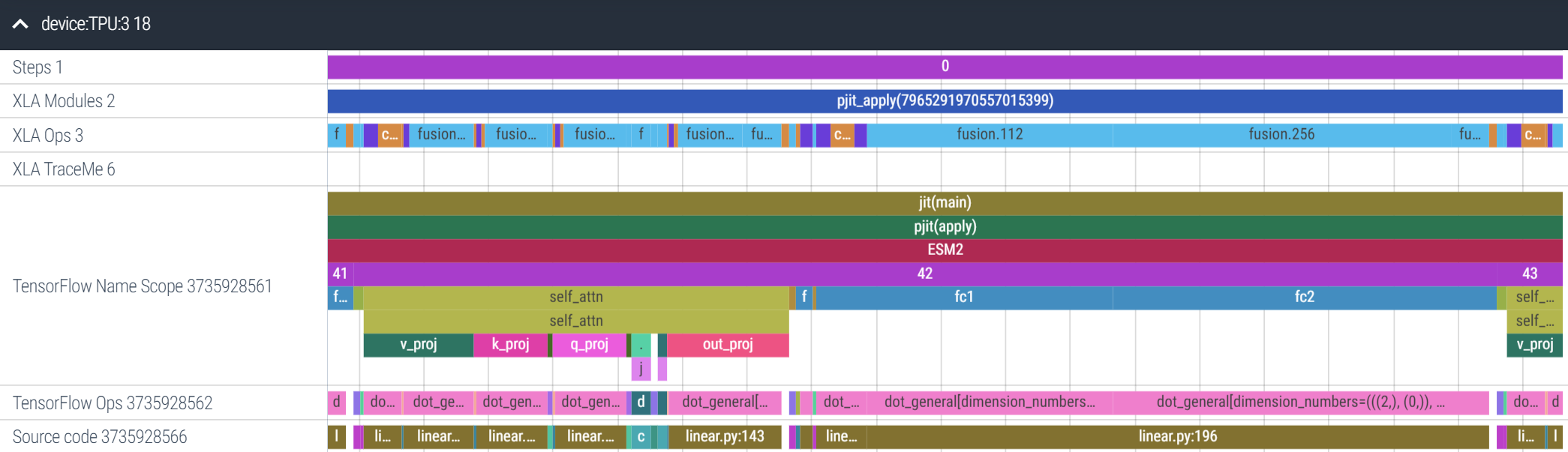
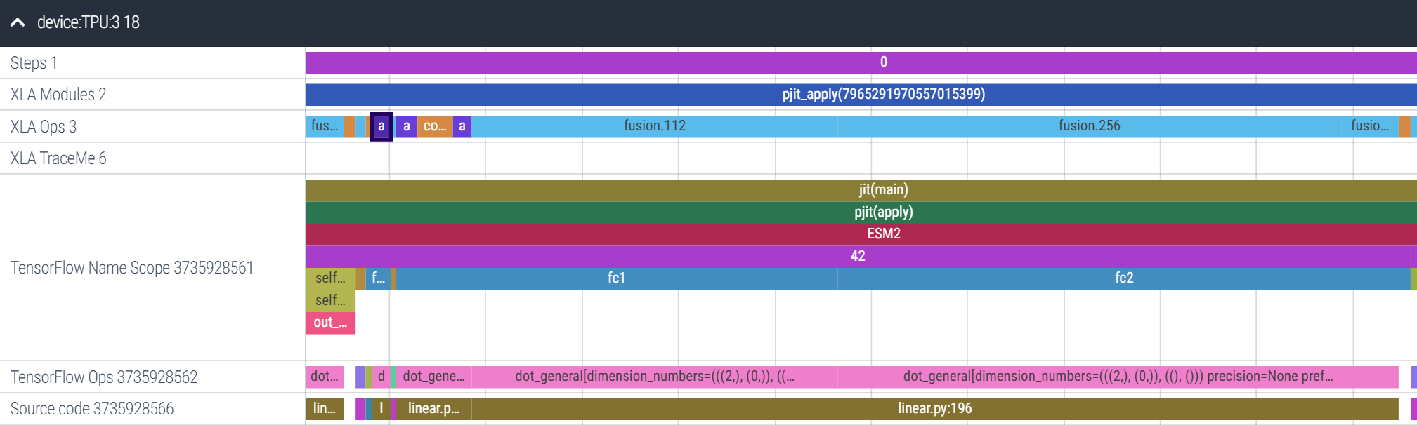
Let’s zoom in more into the FFN sublayer. Amusingly, XLA has decided to allgather fc2’s weight matrix (the selected purple box) before the matmuls of fc1 and fc2. This is the power of JIT-compilation: XLA is able to re-order operations as needed for better performance. It’s also inserted a reduce-scatter over the results (the rightmost, blue fusion op). Overall, the FFN sublayer takes 54ms, and 8ms are spent on collective communication and data reformatting ops, about ~15%¹⁴:

In summary, for a ~20% performance tradeoff, we can now run inference with only one copy of the model stored across all our devices! I want you to explore this trace yourself, so here’s the link to Perfetto; just hit Open trace file and upload this trace, and go play around!

Conclusion: Beyond Tensor Parallelism

Tensor parallelism is powerful, allowing us to scale from 1 GPU/TPU to all 8 connected GPU/TPUs, and when using larger slices of a TPU pod, even further (PaLM was trained using just tensor parallelism, on two full TPUv4 pods with 3072 chips each, Sec. 4). There’s three concluding thoughts I’d like to leave you with:

Pipeline parallelism: Given the large volume of communication involved, tensor parallelism is only viable when there is fast (ideally 1TB/s+) interconnect between devices. This is true for TPUs all the way up to an entire pod; however, GPUs only have fast interconnect (e.g. NVLink) in groups of 8 on a single host. Between hosts, the interconnect is slower (e.g. commercial cloud is typically on the order of ~100GB/s ¹⁵), meaning a different strategy is necessary.

If tensor parallelism is slicing a model “horizontally” (each layer is sharded across all devices), pipeline parallelism is slicing it “vertically” (device 1 can hold layer 0,1 device 2 holds layers 2,3, and so on). The only communication is when activations move between layers, not inside a layer. The problem is that it leads to “bubbles” where devices are inactive (Y. Huang et al., 2019). Large GPU clusters tend to use tensor parallelism for all 8 GPUs connected on a single host, and pipeline parallelism between hosts to make the best of both strategies.

More automation: pjit is incredibly flexible, capable of accommodating any sharding pattern we can come up with. The GSPMD paper covers even more “strange” cases such as sharding convolutions over spatial axes, across multiple devices. However, we still do need to specify a sharding pattern, which for non-experts can be challenging. There’s a lot of exciting work going on in frameworks such as Alpa (Zheng et al., 2022), which automate this entirely, and I’m excited to see where this line of research is headed.
Larger models? Scaling language models has been a strategy that continues to work with no clear signs of slowing down. But a substantial fraction of scaling up goes into learning factual knowledge about the world than the semantics of language. Retrieval-augmented models such as RETRO (Borgeaud et al., 2022) and Atlas (Izacard et al., 2022) are much smaller (the largest RETRO model is only 7.5B params). However, they introduce a new axis (retrieval time) to the current trio of compute, memory use and intra/inter-host communication, and I’m curious to learn where the bottlenecks will arise as this strategy is scaled up.

And factual knowledge can go stale: remember, a BERT model trained in 2019 would associate the word Corona more with beer than the pandemic!

Acknowledgements

Really grateful to Robert Dumitru for reading an early draft of this, providing honest feedback on the bits that “didn’t quite make sense”, and how they could be clearer. Access to TPUs was generously provided through the TPU Research Cloud.

Thanks for taking the time to read through this, and I hope you learned something new! Best place to leave feedback would be either my Twitter, or this form here. See you around!

References

Borgeaud, S., Mensch, A., Hoffmann, J., Cai, T., Rutherford, E., Millican, K., Van Den Driessche, G. B., Lespiau, J.-B., Damoc, B., Clark, A., De Las Casas, D., Guy, A., Menick, J., Ring, R., Hennigan, T., Huang, S., Maggiore, L., Jones, C., Cassirer, A., … Sifre, L. (2022). Improving language models by retrieving from trillions of tokens. In K. Chaudhuri, S. Jegelka, L. Song, C. Szepesvari, G. Niu, & S. Sabato (Eds.), Proceedings of the 39th international conference on machine learning (Vol. 162, pp. 2206–2240). PMLR. https://proceedings.mlr.press/v162/borgeaud22a.html

Bradbury, J., Frostig, R., Hawkins, P., Johnson, M. J., Leary, C., Maclaurin, D., Necula, G., Paszke, A., VanderPlas, J., Wanderman-Milne, S., & Zhang, Q. (2018). JAX: Composable transformations of Python+NumPy programs (Version 0.3.13). http://github.com/google/jax

Chowdhery, A., Narang, S., Devlin, J., Bosma, M., Mishra, G., Roberts, A., Barham, P., Chung, H. W., Sutton, C., Gehrmann, S., Schuh, P., Shi, K., Tsvyashchenko, S., Maynez, J., Rao, A., Barnes, P., Tay, Y., Shazeer, N., Prabhakaran, V., … Fiedel, N. (2022). PaLM: Scaling language modeling with pathways. arXiv. https://doi.org/10.48550/ARXIV.2204.02311

Devlin, J., Chang, M.-W., Lee, K., & Toutanova, K. (2019). BERT: Pre-training of deep bidirectional transformers for language understanding. Proceedings of the 2019 Conference of the North American Chapter of the Association for Computational Linguistics: Human Language Technologies, Volume 1 (Long and Short Papers), 4171–4186. https://doi.org/10.18653/v1/N19-1423

Heek, J., Levskaya, A., Oliver, A., Ritter, M., Rondepierre, B., Steiner, A., & Zee, M. van. (2020). Flax: A neural network library and ecosystem for JAX (Version 0.6.0). http://github.com/google/flax

Huang, A., Subramanian, S., Sum, J., Almubarak, K., & Biderman, S. (2022). The annotated transformer. http://nlp.seas.harvard.edu/annotated-transformer/#encoder-and-decoder-stacks

Huang, Y., Cheng, Y., Bapna, A., Firat, O., Chen, D., Chen, M., Lee, H., Ngiam, J., Le, Q. V., Wu, Y., & Chen, zhifeng. (2019). GPipe: Efficient training of giant neural networks using pipeline parallelism. In H. Wallach, H. Larochelle, A. Beygelzimer, F. dAlché-Buc, E. Fox, & R. Garnett (Eds.), Advances in neural information processing systems (Vol. 32). Curran Associates, Inc. https://proceedings.neurips.cc/paper/2019/file/093f65e080a295f8076b1c5722a46aa2-Paper.pdf

Izacard, G., Lewis, P., Lomeli, M., Hosseini, L., Petroni, F., Schick, T., Dwivedi-Yu, J., Joulin, A., Riedel, S., & Grave, E. (2022). Few-shot learning with retrieval augmented language models. arXiv. https://doi.org/10.48550/ARXIV.2208.03299

Lin, Z., Akin, H., Rao, R., Hie, B., Zhu, Z., Lu, W., Santos Costa, A. dos, Fazel-Zarandi, M., Sercu, T., Candido, S., & Rives, A. (2022). Language models of protein sequences at the scale of evolution enable accurate structure prediction. bioRxiv. https://doi.org/10.1101/2022.07.20.500902

Narayanan, D., Shoeybi, M., Casper, J., LeGresley, P., Patwary, M., Korthikanti, V. A., Vainbrand, D., Kashinkunti, P., Bernauer, J., Catanzaro, B., Phanishayee, A., & Zaharia, M. (2021). Efficient large-scale language model training on GPU clusters using megatron-LM. arXiv. https://doi.org/10.48550/ARXIV.2104.04473

Rajbhandari, S., Rasley, J., Ruwase, O., & He, Y. (2020). ZeRO: Memory optimizations toward training trillion parameter models. Proceedings of the International Conference for High Performance Computing, Networking, Storage and Analysis.

Roberts, A., Chung, H. W., Levskaya, A., Mishra, G., Bradbury, J., Andor, D., Narang, S., Lester, B., Gaffney, C., Mohiuddin, A., Hawthorne, C., Lewkowycz, A., Salcianu, A., Zee, M. van, Austin, J., Goodman, S., Soares, L. B., Hu, H., Tsvyashchenko, S., … Gesmundo, A. (2022). Scaling up models and data with \(\texttt{t5x}\) and \(\texttt{seqio}\). arXiv Preprint arXiv:2203.17189. https://arxiv.org/abs/2203.17189

Shoeybi, M., Patwary, M., Puri, R., LeGresley, P., Casper, J., & Catanzaro, B. (2019). Megatron-LM: Training multi-billion parameter language models using model parallelism. arXiv. https://doi.org/10.48550/ARXIV.1909.08053

Vaswani, A., Shazeer, N., Parmar, N., Uszkoreit, J., Jones, L., Gomez, A. N., Kaiser, Ł., & Polosukhin, I. (2017). Attention is all you need. In I. Guyon, U. V. Luxburg, S. Bengio, H. Wallach, R. Fergus, S. Vishwanathan, & R. Garnett (Eds.), Advances in neural information processing systems (Vol. 30). Curran Associates, Inc. https://proceedings.neurips.cc/paper/2017/file/3f5ee243547dee91fbd053c1c4a845aa-Paper.pdf

Weng, L. (2021). How to train really large models on many GPUs? Lilianweng.github.io. https://lilianweng.github.io/posts/2021-09-25-train-large/

Xu, Y., Lee, H., Chen, D., Hechtman, B. A., Huang, Y., Joshi, R., Krikun, M., Lepikhin, D., Ly, A., Maggioni, M., Pang, R., Shazeer, N., Wang, S., Wang, T., Wu, Y., & Chen, Z. (2021). GSPMD: General and scalable parallelization for ML computation graphs. CoRR, abs/2105.04663. https://arxiv.org/abs/2105.04663

Yoo, J., Perlin, K., Kamalakara, S. R., & Araújo, J. G. M. (2022). Scalable training of language models using JAX pjit and TPUv4. arXiv. https://doi.org/10.48550/ARXIV.2204.06514

Zheng, L., Li, Z., Zhang, H., Zhuang, Y., Chen, Z., Huang, Y., Wang, Y., Xu, Y., Zhuo, D., Xing, E. P., Gonzalez, J. E., & Stoica, I. (2022). Alpa: Automating inter- and Intra-Operator parallelism for distributed deep learning. 16th USENIX Symposium on Operating Systems Design and Implementation (OSDI 22), 559–578. https://www.usenix.org/conference/osdi22/presentation/zheng-lianmin

Footnotes

and a copy of the optimizer state and gradients when we’re training, so potential total memory use of upto 3x the size of the model itself.↩︎
Specifically, in section 5.2 the authors note “We trained our models on one machine with 8 NVIDIA P100 GPUs.”↩︎
Why the row vectors of \(A\) and the column vectors of \(B\)? Why not just the column vectors of both? This is mostly due to convention, as confusing as it can be for newcomers. I like the Mnemonic RAC-B (“rack b”), rows of A, columns of B.↩︎
For an \(N \times N\) matrix, matrix multiplication has time complexity \(O(N^3)\) while matrix addition is \(O(N^2)\). For a large enough matrix, the speedup from the parallel matrix multiplies can outweigh the cost of communicating then adding afterwards.↩︎
You may also recognize this as just jax.lax.psum, which it is!↩︎
Of course, not accounting for the communication overhead of the AllReduce. For systems that are compute-bound, splitting the actual multiplication across multiple devices and syncing them together (due to the \(O(N^3)\) compute costs of a matrix multiply vs the \(O(N^2)\) memory transfer) is still often worth it.↩︎
Again, the outer axes in a matrix multiply are individual vectors; the inner axes are the feature dimensions of those vectors, as we saw in the intro. Feel free to scroll back if you need to recap!↩︎
Note that in math contexts this is often written as \(Wx\), where \(x\) is a column vector. In Python, data points are stored as row vectors, which means \(X\) has to be on the left hand side (because the feature dimension needs to be the inner dimension, the one we take dot products over!).↩︎
Roughly speaking. The dot product is sensitive to the magnitude of the vectors too, not just their direction. If a particular weight vector is very large, it will have large dot products even if the data vector isn’t that similar. However, with proper regularization, most weight vectors should be within a “reasonable” range, enabling comparison.↩︎
This is specifically the “2D finalized” sharding pattern presented in Table 1.↩︎
Or in the math textbook way, “this is left as an exercise to the reader”. But really, I think working it out would be a neat exercise!↩︎
On a larger model, we’d shard even the biases and layer norms, but on this scale it’s fine not to. They’re a lot smaller than the weights.↩︎
A quick estimate counting both the communication ops (e.g. allgather, fused reduce-scatters) as well as data formatting ops.↩︎
It’s worse in the self-attention sublayer (29%), which also takes less time overall, resulting in an average of 20%. Would be a better layer to focus more for improvement!↩︎
Although, newer offerings such as the p4d.24xlarge or BM.GPU4.8 have considerably better inter-node bandwidth. At the same time, the A100 GPUs themselves are much faster, which means the inter-node bandwidth must keep up just to avoid becoming a bottleneck.↩︎

Tensor Parallelism with `jax.pjit`

Intro: Parallelism

Data Parallelism

Tensor Parallelism

Partitioning: Intuition

Intro: Dot products

Intro: Matrix multiplies

Sharding: A Matrix Multiply

Case 1: Inner Axes

Case 1A: Mesh-axes match

Multiply

AllReduce

Case 1B: Mesh-axes mismatch

Case 2: Outer Axes

Full Sharding

Sharding: GSPMD-style

What is \(XW\)?

GSPMD’s sharding spec

Embed \(\rightarrow\) Hidden

Hidden \(\rightarrow\) Embed

Wrapping it up

Partitioning: In JAX

The `pjit` programming model

Sharding constraints

A first run

Applying constraints to a FFN

Sharding constraints: Weights

Putting it all together

Program Trace

Conclusion: Beyond Tensor Parallelism

Further Reading

Acknowledgements

References

Footnotes

Intro: Parallelism

Data Parallelism

Tensor Parallelism

Partitioning: Intuition

Intro: Dot products

Intro: Matrix multiplies

Sharding: A Matrix Multiply

Case 1: Inner Axes

Case 1A: Mesh-axes match

Multiply

AllReduce

Case 1B: Mesh-axes mismatch

Case 2: Outer Axes

Full Sharding

Sharding: GSPMD-style

What is \(XW\)?

GSPMD’s sharding spec

Embed \(\rightarrow\) Hidden

Hidden \(\rightarrow\) Embed

Wrapping it up

Partitioning: In JAX

The pjit programming model

Sharding constraints

A first run

Applying constraints to a FFN

Sharding constraints: Weights

Putting it all together

Program Trace

Conclusion: Beyond Tensor Parallelism

Further Reading

Acknowledgements

References

Footnotes

The `pjit` programming model