Code
import plotly.express as px
from plotly.subplots import make_subplots
import plotly.graph_objects as go

import numpy as npSpherical harmonics are powerful mathematical tools, allowing us to represent any function on a sphere as the sum of simpler basis functions (much like a Fourier series!). This post aims to explain spherical harmonics through the lens of Fourier series, by “lifting” them from a circle to a sphere, extensively relying on visual explanations.
import plotly.express as px
from plotly.subplots import make_subplots
import plotly.graph_objects as go
import numpy as npSuppose we have a periodic function \(f(\theta)\), with a period \(2\pi\). As an example, let \(f(\theta) = \sin(\theta) - 0.5\cos(2\theta) + 0.25\sin(3\theta)\). This is the standard way to view the function: angle \(θ\) on the x-axis, \(f(θ)\) on the y-axis.
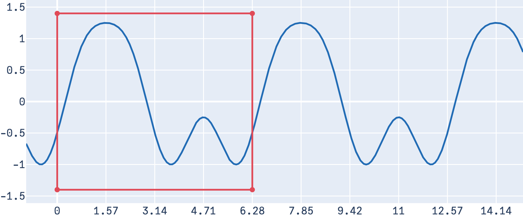
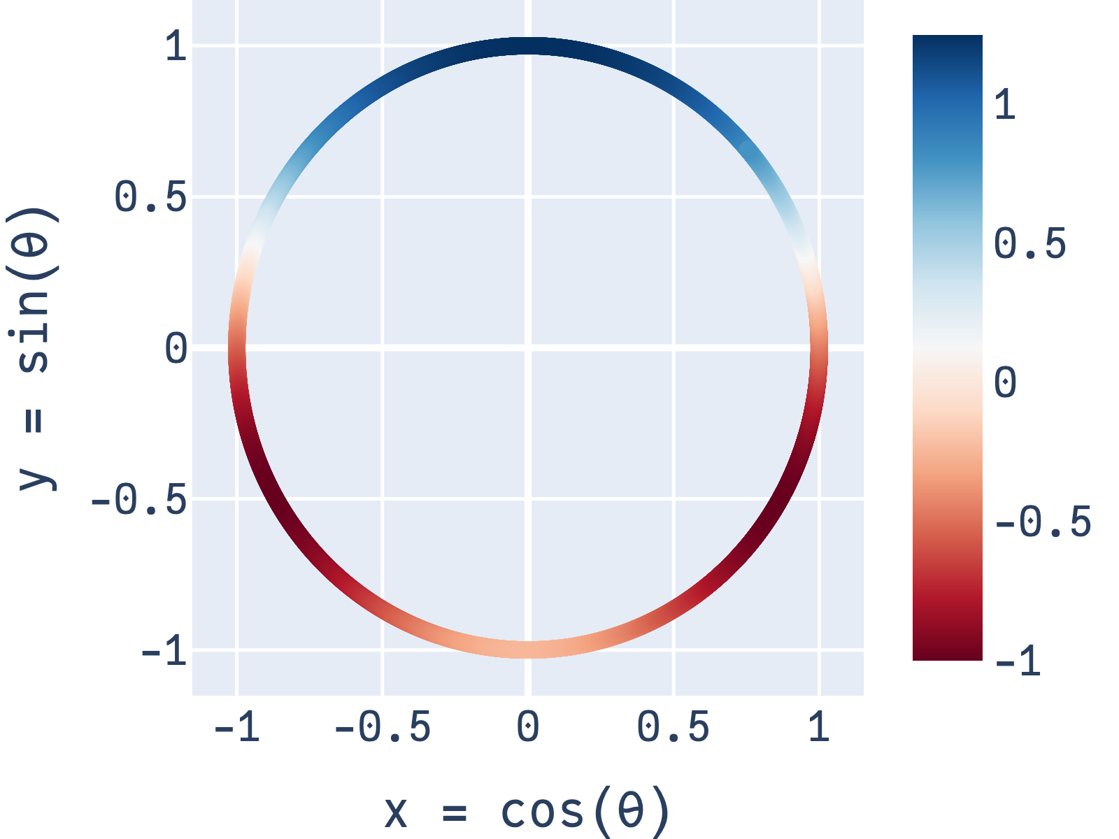
Since the function is periodic, there is an equivalent way to view this: as a function defined on a circle with radius 1 (and in turn, a circumference of 2π). The period here is represented counter-clockwise (as is convention in trigonometry). Just as in the previous plot, we can see that the function first rises to a large “hill”, before descending into two small “valleys”, returning to the starting point.
One of the most widely used discoveries in mathematics is that any real-valued, periodic function1 can be represented as the weighted sum of sines and cosines2 of varying frequencies, called a Fourier Series. Specifically, for a function with a period of \(2\pi\), there exists weights \(a_n\) (weights for the cosines) and \(b_n\) (weights for the sines) such that:
\[f(\theta) = \frac{a_0}{2} + \sum_{n=1}^\infty a_n \cos(n\theta) + b_n \sin(n\theta)\]
The process of finding the exact weights belong to the study of Fourier Analysis. In our case, since the function we’ve chosen is already neatly written as a sum of sines and cosines, \(f(\theta) = \sin(\theta) - 0.5\cos(2\theta) + 0.25\sin(3\theta)\), the weights can be read off directly: \(b_1 = 1\), \(a_1 = -0.5\) and \(b_3 = 0.25\); all the other weights are zero3. We can also visualize \(f(θ)\) with the relevant sine and cosine functions (a.k.a the “basis functions”)4.
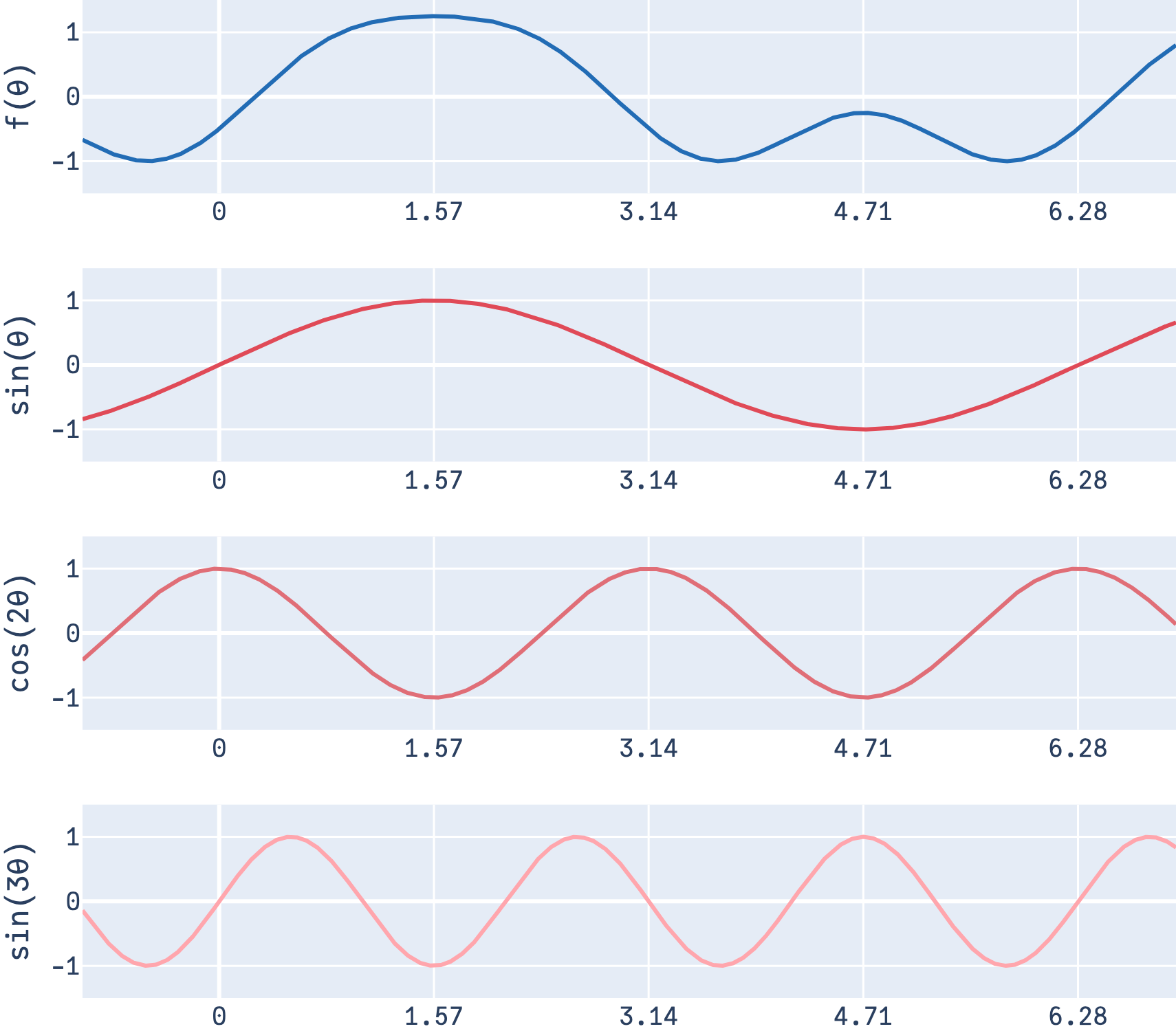
Note that for a finite number of terms, this is exact only when the function can be expressed in terms of sines and cosines; otherwise (with function such as say, a square wave) this only exact when the sum uses an infinite number of terms.
Looping back5 to earlier, these basis functions can also be represented on a circle:
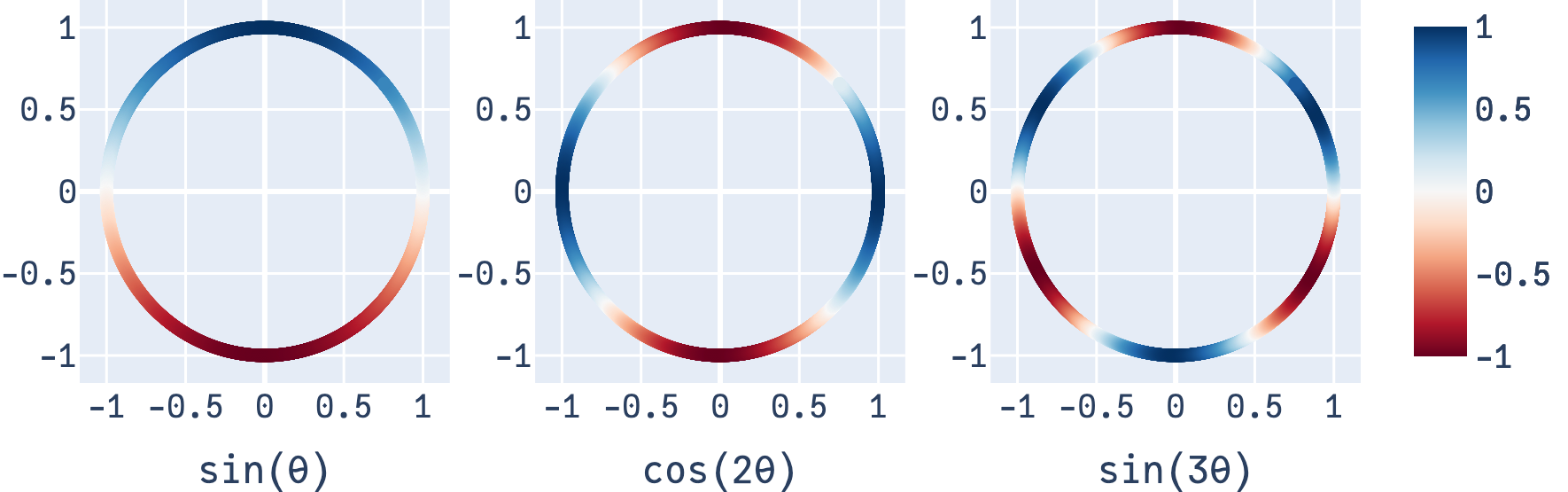
The takeaway here is that even though the circle plots look very different from the standard plot (with \(θ\) on the x-axis), they’re simply two different ways of depicting the exact same function on a circle.
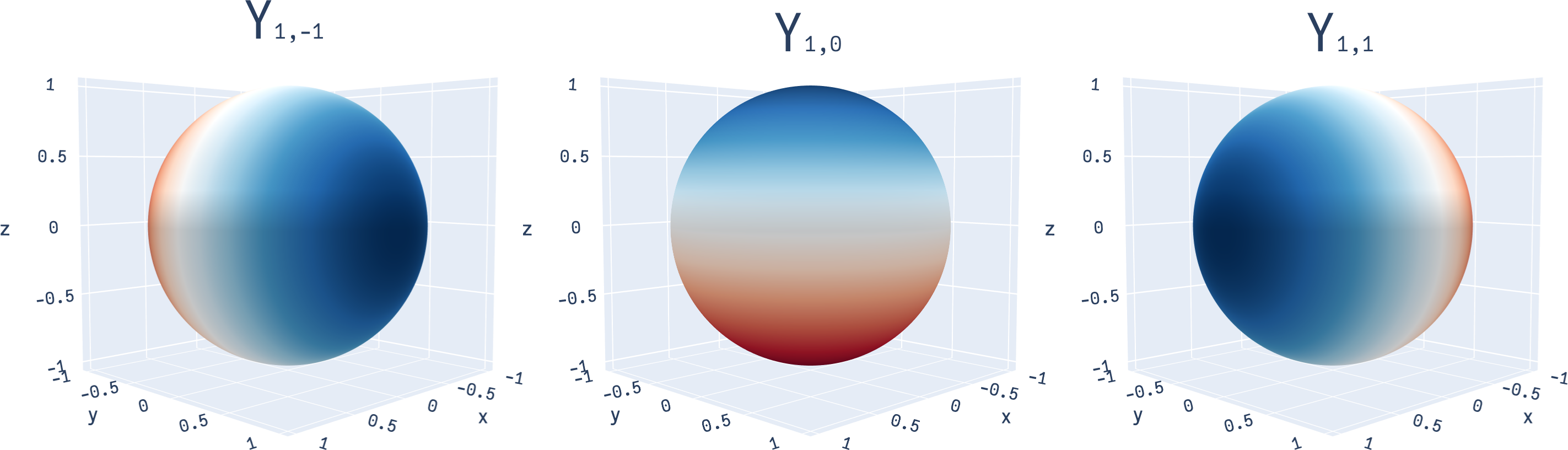
If you’ve followed the visuals so far, you already know what a spherical harmonic is: instead of basis functions defined on a circle, they’re basis functions defined on a sphere 6. Just like how \(\sin(\theta)\) forms a function on a circle, the spherical harmonics are functions on a sphere. Here’s one (it’s interactive!):
fig = make_subplots(rows=1, cols=1, specs=[[{'is_3d': True}]])

s = np.linspace(0, 2 * np.pi, 100)
t = np.linspace(0, np.pi, 100)
tGrid, sGrid = np.meshgrid(s, t)

r = 1
x = r * np.cos(sGrid) * np.sin(tGrid)
y = r * np.sin(sGrid) * np.sin(tGrid)
z = r * np.cos(tGrid)


fig.add_trace(
  go.Surface(x=x, y=y, z=z,
    surfacecolor=np.sqrt(3/4*np.pi)*y,
    colorscale='RdBu',
    colorbar=dict(thickness=10)
  )
)

fig.update_layout(
    font_family="JuliaMono",
    showlegend=False,
    margin=go.layout.Margin(l=0, r=0, b=0, t=0),
    paper_bgcolor='rgba(0,0,0,0)',
)

fig.update_traces(showscale=False)
fig.show()On the circle, Fourier Analysis allows us to convert any function defined on a circle (i.e. a periodic function) into the weighted sum of sines and cosines of varying frequencies. Now, on the sphere, any function on a sphere can be decomposed into a weighted sum of the spherical harmonic functions \(Y_{lm}\). That is, there exist \(a_{lm}\) such that:
\[ \begin{align*} f(x, y, z) &= \sum_{l=0}^\infty \sum_{m=-l}^l a_{lm} Y_{lm}(x,y,z) \\ &\text{where } x^2+y^2+z^2 = 1 \end{align*} \]
There’s a few things to note here:
Real vs Complex: Both indices are subscripts on \(Y\), i.e. of the form \(Y_{lm}\). This convention reflects that we’re looking at the real spherical harmonics here (complex ones have indices of the form \(Y_l^m\))
Coordinates: Note that we’re using cartesian coordinates (x, y, z) as inputs to the spherical harmonics, not angles. We could equivalently use harmonics of the form \(Y_{lm}(\theta, \phi)\) to stay consistent with the Fourier series, but they’re simpler in cartesian form (and as we’ll see in a bit, equivalent).
Often, spherical harmonics are not depicted on the sphere directly, but in a different form. For instance, in the alternate depiction \(Y_{1, -1}\) looks as such:
fig = make_subplots(rows=1, cols=1,
                    specs=[[{'is_3d': True}]])

theta = np.linspace(0, np.pi, 100)
phi = np.linspace(0, 2*np.pi, 100)
theta, phi = np.meshgrid(theta, phi)

x = np.sin(theta) * np.cos(phi)
y = np.sin(theta) * np.sin(phi)
z = np.cos(theta)

r0a = np.sqrt(3/4*np.pi)*y
r0 = np.abs(r0a)
fig.add_trace(
  go.Surface(
    x=r0*x, y=r0*y, z=r0*z,
    surfacecolor=r0a,
    colorscale='RdBu'
  )
)


fig.update_layout(
    font_family="JuliaMono",
    showlegend=False,
    margin=go.layout.Margin(l=0, r=0, b=0, t=0),
    paper_bgcolor='rgba(0,0,0,0)',
)

fig.update_layout(
  scene = dict(
    xaxis = dict(nticks=4, range=[-1.8,1.8],),
    yaxis = dict(nticks=4, range=[-1.8,1.8],),
    zaxis = dict(nticks=4, range=[-1.8,1.8],)
  ),
  scene1_aspectratio=dict(x=1, y=1, z=1)
)

fig.update_traces(showscale=False)
fig.show()Note that while it appears that \(Y_{1, -1}\) is defined over two mini-spheres, this is incorrect! The harmonic is still defined over the sphere; this plot simply represents it in a different way. Previously, we plotted a surface through all points on the sphere, that is:
\[ \{\hspace{0.2cm} \mathbf{x} \hspace{0.2cm} \bigl\vert \hspace{0.2cm} \| \mathbf{x} \|_2 = 1\} \]
Now, we’re plotting a surface through all points:
\[ \{\hspace{0.2cm} \mathbf{x} \lvert f(\mathbf{x}) \rvert \hspace{0.2cm} \bigl\vert \hspace{0.2cm} \| \mathbf{x} \|_2 = 1\} \\ \]
Specifically, we allow the magnitude of the function \(\lvert f(x,y,z) \rvert\) to modulate how far the point on the surface in that direction is from the origin. When the magnitude is small, the surface is “shrunk” closer to the origin; where it’s large, it is “expanded” away from the origin, such that the distance to the origin is the magnitude of the function in that direction. The surface is still colored by value; here, blue still represents positive values, red represents negative values.
As we can see, on the plane \(y=0\) (where \(Y_{1, -1} = 0\)), the points have indeed been shrunk directly to the origin. Note the underlying function is the exact same; only thing changed is how we visualize it.
To really visually grasp this, it’s helpful to drop back down to the 2D case. Let’s do the shrink and expand procedure we just described to \(\sin(\theta)\). We end up with the following plot. Remember, this is only a visual aid, \(\sin(\theta)\) is still only defined on the circle and the left is the “true” plot.
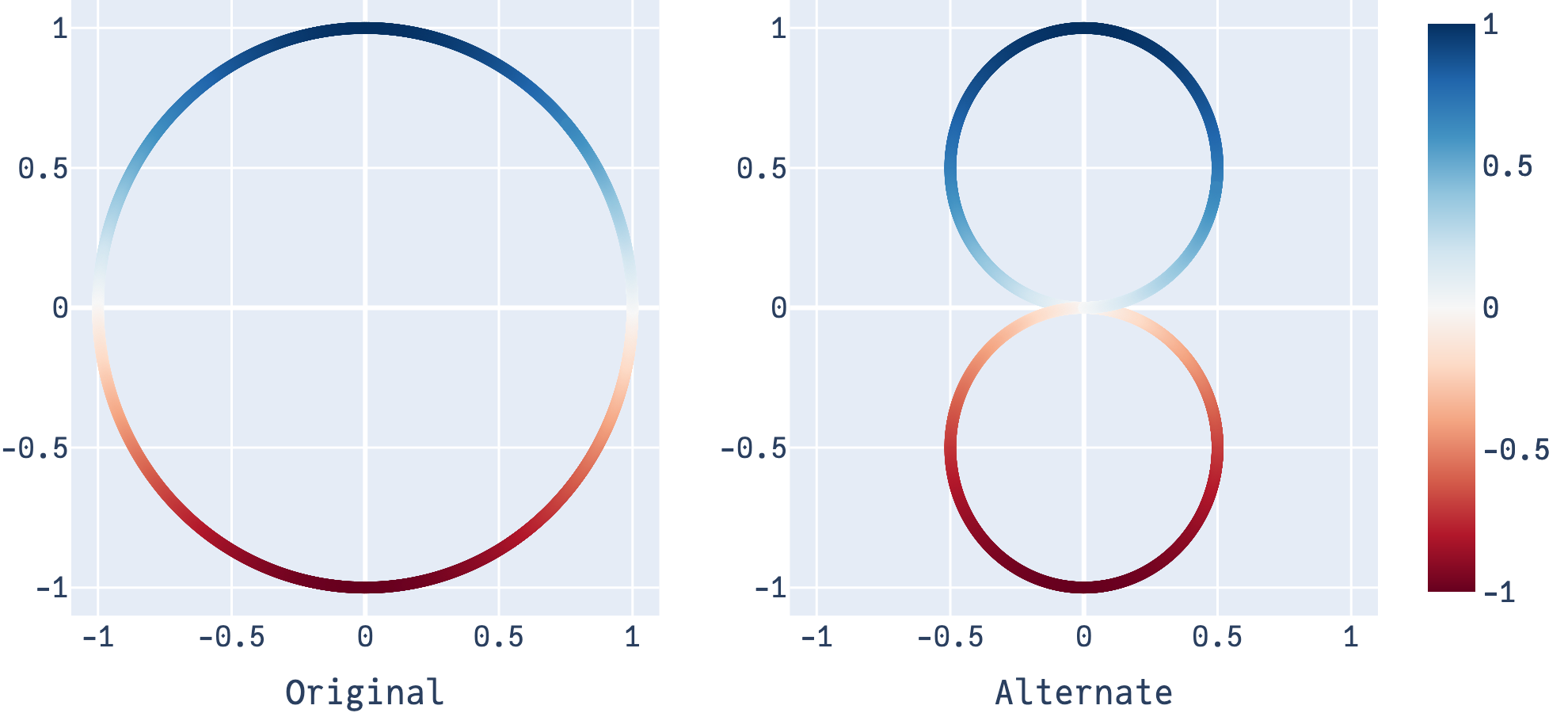
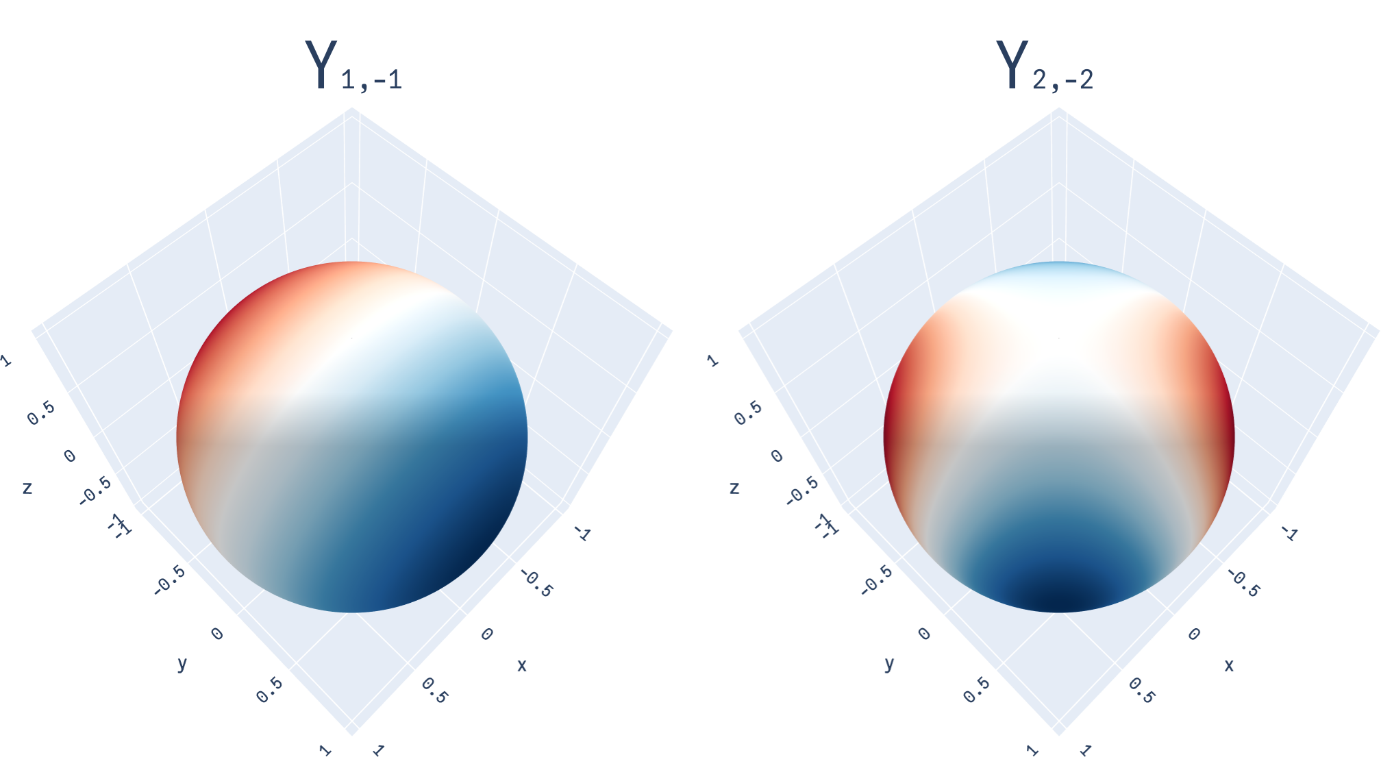
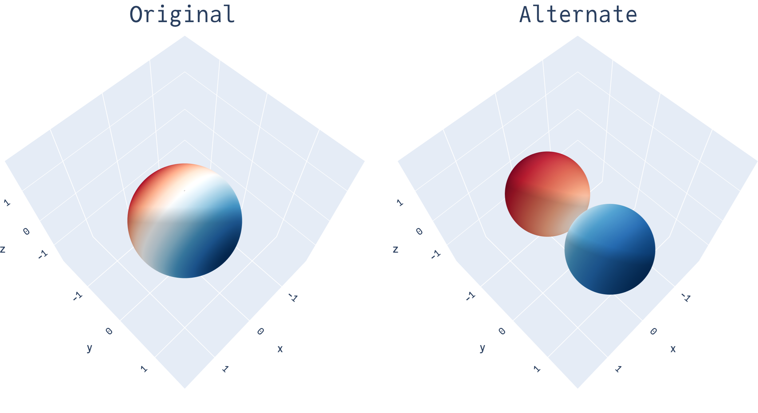
Completing the visual analogy, here’s the original and alternate version diagrams for \(Y_{1, -1}\) side-by-side:
The alternate visual depiction of the harmonics may seem needlessly complicated at first. But they serve an important purpose: as the harmonics become more complex as the degree goes up and we begin linearly combining them together, the alternate form allows a clearer depiction of how different values of the function on the sphere compare to each other. For example, here’s \(Y_{4, 0} + 2Y_{2, -1}\):
fig = make_subplots(rows=1, cols=1,
                    specs=[[{'is_3d': True}]])

theta = np.linspace(0, np.pi, 100)
phi = np.linspace(0, 2*np.pi, 100)
theta, phi = np.meshgrid(theta, phi)

x = np.sin(theta) * np.cos(phi)
y = np.sin(theta) * np.sin(phi)
z = np.cos(theta)

r0a = 3/16*np.sqrt(1/np.pi)*(35*z**4-30*z**2+3) + 2*(1/2*np.sqrt(15/np.pi)*y*z)
r0 = np.abs(r0a)

fig.add_trace(
  go.Surface(
    x=r0*x, y=r0*y, z=r0*z,
    surfacecolor=r0a,
    colorscale='RdBu'
  )
)


fig.update_layout(
    font_family="JuliaMono",
    showlegend=False,
    margin=go.layout.Margin(l=0, r=0, b=0, t=0),
    paper_bgcolor='rgba(0,0,0,0)',
)

fig.update_layout(
  scene = dict(
    xaxis = dict(nticks=4, range=[-1.8,1.8],),
    yaxis = dict(nticks=4, range=[-1.8,1.8],),
    zaxis = dict(nticks=4, range=[-1.8,1.8],)
  ),
  scene1_aspectratio=dict(x=1, y=1, z=1)
)

camera = dict(eye=dict(x=1.5, y=1.5, z=1.5))
fig.layout.scene1.camera = camera

fig.update_traces(showscale=False)
fig.show()You may have noticed I’ve been referring to the harmonics by their degree and order (such as \(Y_{1,1}\)), but not their exact algebraic forms. Unlike the Fourier series (where each of the \(n^{th}\) sine and cosine terms are simply \(\sin(n\theta)\) and \(\cos(n\theta)\)), the spherical harmonics are a more complex set of functions7; here’s some of them8:
\[ \begin{align*} Y_{00}(x, y, z) &= \frac{1}{2} \sqrt{\frac{1}{\pi}} \\ Y_{1, -1}(x, y, z) &= \sqrt{\frac{3}{4\pi}} y \\ Y_{3, -2}(x, y, z) &= \frac{1}{2}\sqrt{\frac{105}{\pi}} xyz \\ \end{align*} \]
These are the Cartesian versions of the spherical harmonics, but it is important to know that conventions vary significantly across fields (for instance, the quantum mechanics community implictly places a factor of \((-1)^m\) in every harmonic, whereas the magnetics community does not). It is well advised to check which version of the harmonics are being used in a specific application.
To get a version of the harmonics in spherical coordinates (to get something akin to terms in the Fourier series), all one has to do is apply the standard change of basis formula9:
\[ \begin{align*} x &= \sin(\theta) \cos(\phi) \\ y &= \sin(\theta) \sin(\phi) \\ z &= \cos(\theta) \end{align*} \]
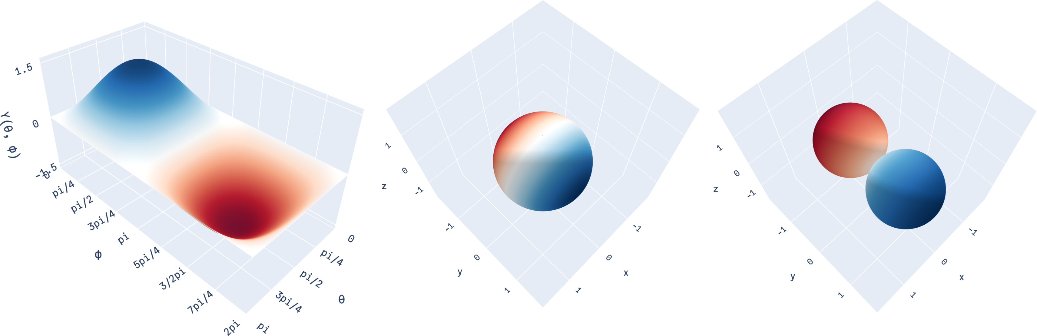
As an example, \(Y_{1, -1}\) now becomes \(Y_{1, -1}(\theta, \phi) = \sqrt{\frac{3}{4\pi}} \sin(\theta) \sin(\phi)\). We could plot this function on the 2D plane10, just as we plotted \(\sin(\theta)\) on the 1D line at the start of this article:
fig = make_subplots(rows=1, cols=1,
                    specs=[[{'is_3d': True}]])

theta = np.linspace(0, 2*np.pi, 100)
phi = np.linspace(0, 2*np.pi, 100)
theta, phi = np.meshgrid(theta, phi)

x = np.sin(theta) * np.cos(phi)
y = np.sin(theta) * np.sin(phi)
z = np.cos(theta)

r0a = np.sqrt(3/4*np.pi) * np.sin(theta) * np.sin(phi)
# r0 = np.abs(r0a)
fig.add_trace(
  go.Surface(x=theta, y=phi, z=r0a,
    surfacecolor=r0a,
    colorscale='RdBu'
  )
)

fig.update_layout(
    font_family="JuliaMono",
    showlegend=False,
    margin=go.layout.Margin(l=0, r=0, b=0, t=0),
    paper_bgcolor='rgba(0,0,0,0)',
)

fig.update_layout(
  scene = dict(
    xaxis = dict(
      tickvals=[0, np.pi/4, np.pi/2, 3*np.pi/4, np.pi],
      ticktext=['0', 'pi/4', 'pi/2', '3pi/4', 'pi'],
      range=[0,np.pi],
      title_text="θ"),
    yaxis = dict(
      tickvals=[0, np.pi/4, np.pi/2, 3*np.pi/4, np.pi, 5*np.pi/4, 6*np.pi/4, 7*np.pi/4, 8*np.pi/4],
      ticktext=['0', 'pi/4', 'pi/2', '3pi/4', 'pi', '5pi/4', '3/2pi', '7pi/4', '2pi'],
      nticks=4,
      range=[0,2*np.pi],
      title_text="ϕ"),
    zaxis = dict(
      title_text="Y(θ, ϕ)",
      nticks=3,
      tickvals=[-1.5, 0, 1.5])),
  scene1_aspectratio=dict(x=1, y=2, z=1),
  margin=dict(r=20, l=10, b=10, t=10)
)

camera = dict(eye=dict(x=2, y=2, z=2))
fig.layout.scene1.camera = camera

fig.update_traces(showscale=False)
fig.show()Just as how we were able to interpret a periodic function on the 1D line as being on a circle, we can now see certain periodic functions on the 2D plane as existing on a sphere11. This now also means we have three different ways of looking at periodic functions on circles and spheres!
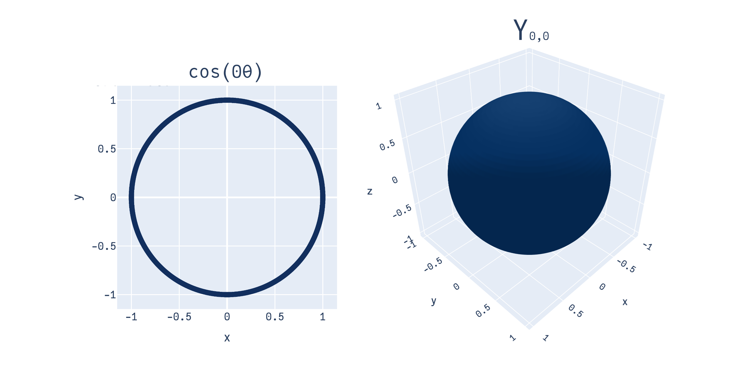
Firstly, in the 1D case, we can represent \(\sin(\theta)\) as:
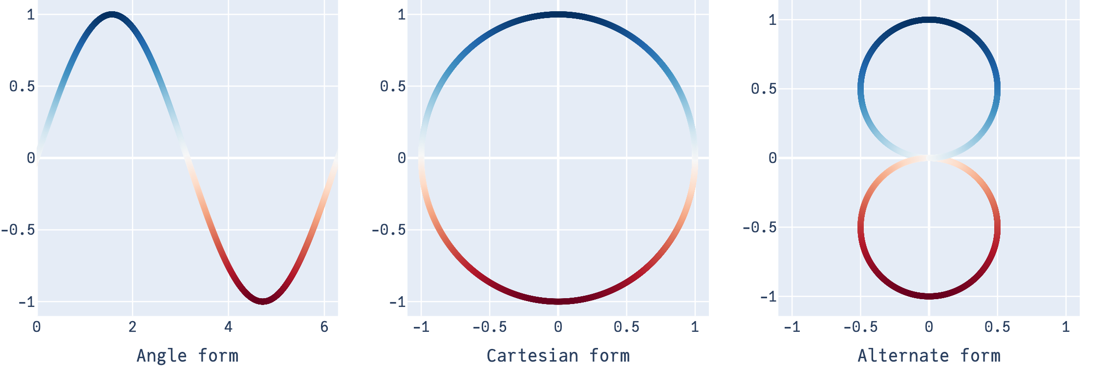
Similarly, in the 2D case, we can represent \(Y_{1,-1}\) as:
Now that we’ve finished making the connection between the Fourier series and Spherical harmonics, one might ask: what are they actually used for? There’s plenty (they pop up rather frequently when functions on a sphere are involved), here are some:
Solving PDEs: Recall that the motivating reason behind the discovery of the Fourier series was to solve the heat equation, which is a partial differential equation. Likewise, we can now decompose any (well-behaved) function on a sphere into a sum of spherical harmonics as basis functions, and solve the PDE using these basis functions (instead of the more complicated original)
Physics: One particularly important PDE is Schrödinger’s equation. Focusing on hydrogen-like atoms, the spherical harmonics can be use to describe the angular component of the solutions, which can then be converted into the probability that the electron will be found in a specific direction. Note that the angular component cannot tell us the probability how far from the origin the electron will be found (that’d be the radial component), only the probability in a given direction.
Machine Learning: One problem with ordinary neural networks is that they do not respect input geometry. For example, if your input is a molecule (with atom coordinates) and your output is toxicity, if you rotate the input, the hidden layer outputs will change in an ill-defined way and return a different prediction, even though your input is the same molecule! Spherical harmonics are used to build rotationally equivariant neural networks, such that the change for a rotation properly is defined, and then ultimately produce an invariant prediction: predicting the same toxicity level for a molecule, regardless of input orientation.
Spherical harmonics were one of those things that felt intimidating to me at first, because of the dense math involved. But ultimately, they’re basically a sibling of the Fourier series, the only difference being that they’re for functions defined on a sphere instead of a circle. The math, once visualized, is beautiful, and I hope this has been a helpful read!
Appendix B, Spherical Harmonics: This chapter from Wojciech Jarosz’s Ph.D. dissertation is a great resource on spherical harmonics, particularly the real-valued ones (it’s written from a computer graphics standpoint; most physics-oriented ones would focus on the complex-valued ones).
e3nn library: This PyTorch library is geared toward equivariant neural networks broadly, but also contains optimized implementations to compute spherical harmonics.
SEGNNs paper: This is a recent paper on constructing equivariant neural networks; the appendix has a great section on how spherical harmonics are used to build them.
Or more broadly, even nonperiodic and/or complex-valued functions. We’re not taking a look at them here, but for a deeper dive there’s this great 3b1b video.↩︎
There are many different conventions on how to represent fourier series (such as the amplitude-phase form, the exponential form, etc.), which you can find here. We’re using the sine-cosine form for this article.↩︎
The curious reader could verify this directly! Each coefficient is defined as the integral over the period (here, \(0\) to \(2π\)) of the product of the function \(f(θ)\) and the trigonometric function. For example, from \(0\) to \(2π\), \(\int f(\theta)sin(3\theta)d\theta = 0.25\)↩︎
They’re called basis functions, as a linear combination of these functions can produce any periodic function; akin to how a linear combination of a basis in \(\mathbb{R}^3\) (e.g. \([1,0,0]\), \([0,1,0]\) and \([0,0,1]\)) can produce any vector in R³.
More formally, these infinitely many sine and cosine functions together form a basis for “square-integrable” functions defined on the circle, that is, for \(L_2({S^1})\).↩︎
Terrible pun absolutely intended.↩︎
More precisely, they form a basis for \(L_2(S^2)\), the space of square integrable functions defined on the sphere.↩︎
This also means in practice, efficient calculation of the values are non-trivial, since there are so many different functions to account for. The functions themselves are not arbitrary; they’re made of the derivatives of Legendre polynomials of varying degrees.↩︎
A more exhaustive table of them can be found on Wikipedia here. Note that we’re assuming r=1 throughout this article.↩︎
For a recap of Spherical coordinates, this may be helpful. Note that there’s multiple conventions! We’re using the physics convention here (in the math one, \(ϕ\) and \(θ\) are flipped).↩︎
Note that we plot \(ϕ\) from \(0\) to \(2π\), but \(θ\) only from \(0\) to \(π\); this covers the whole sphere. This is because \(θ\) can be seen as selecting the “height” on the sphere, and then we traverse a full cycle (with \(ϕ\)) on the circle at that height. \(θ\) being from \(0\) to \(π\) is enough, otherwise we’d use each height twice.↩︎
Note for this to hold, the values on the entire boundary must be the same (not just the endpoint as in the 1D case), as they get mapped to one of the two poles on the sphere; here all points on the boundary have the value 0.
For a more general periodic function (where the entire boundary doesn’t have the same value), where the period endpoints of any 1D slice (parallel to the x or y axes) of the 2D function are the same, it is possible to see that function existing on a torus, that is, \(L_2(S^1 \times S^1)\) instead of \(L_2(S^2)\).↩︎